Exploring the Graph of X Cosx function reveals a capture interplay between linear and trigonometric components. This office combines a uncomplicated linear term with the cosine mapping, creating a singular and visually scheme graph. Understanding the Graph of X Cosx involves dig into the properties of both linear and cosine functions and how they interact to form a composite graph.
Understanding the Components
The Graph of X Cosx is pen of two chief components: the linear function x and the cosine mapping cos (x). Let's break down each component to understand their case-by-case characteristics before combining them.
Linear Function: x
The linear mapping x is a straightforward map where the output is direct proportional to the input. Its graph is a straight line legislate through the origin with a slope of 1. This function is continuous and increases linearly as x increases.
Cosine Function: cos (x)
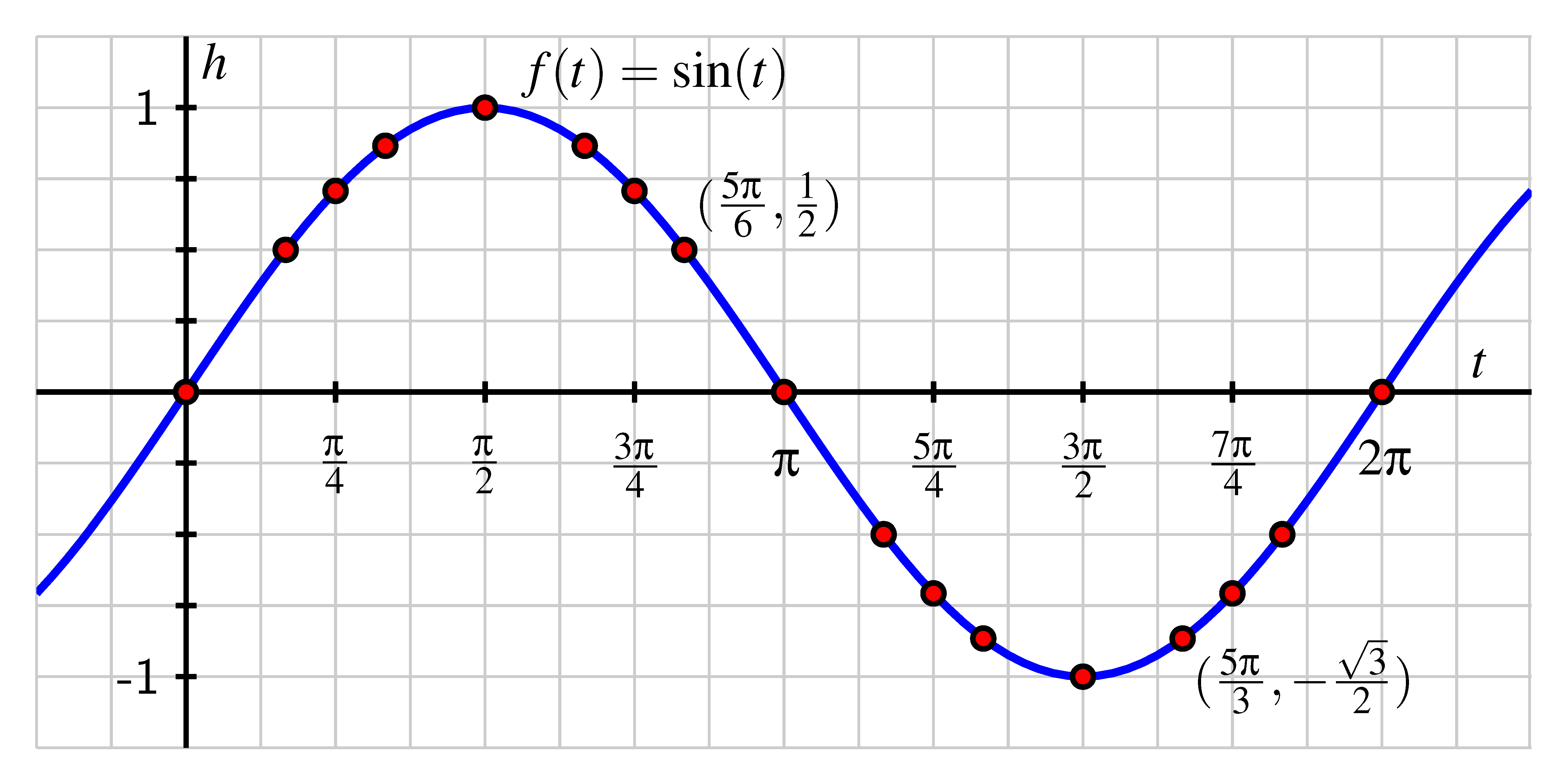
The cosine use, cos (x), is a occasional function that oscillates between 1 and 1. It has a period of 2π, meaning it repeats its values every 2π units. The graph of cos (x) is a smooth, wavy line that crosses the x axis at multiples of π and reaches its maximum and minimum values at 2nπ and (2n 1) π, respectively, where n is an integer.
Combining the Functions
When we combine the linear function x and the cosine part cos (x), we get the function f (x) x cos (x). This combination results in a graph that exhibits both linear growth and occasional oscillations. The linear term x causes the graph to rise steadily, while the cosine term cos (x) introduces periodic fluctuations.
Graphical Characteristics
The Graph of X Cosx has various notable characteristics:
- Asymptotic Behavior: As x approaches positive or negative eternity, the linear term x dominates, causing the graph to approach a straight line with a slope of 1.
- Periodic Oscillations: The cosine term introduces periodical oscillations around the linear trend. These oscillations have an amplitude of 1 and a period of 2π.
- Intersection Points: The graph intersects the x axis at points where x cos (x) 0. These points occur periodically and can be found by lick the equating.
Analyzing the Graph
To gain a deeper understanding of the Graph of X Cosx, let's analyze it in different intervals and observe how the linear and cosine components interact.
Interval Analysis
Consider the interval [0, 2π]. Within this interval, the cosine use completes one total cycle, hover from 1 to 1 and back to 1. The linear term x increases steady from 0 to 2π. The compound function f (x) x cos (x) will show a climb trend with superimpose oscillations.
for instance, at x 0, f (0) 0 cos (0) 1. At x π, f (π) π cos (π) π 1. At x 2π, f (2π) 2π cos (2π) 2π 1. These points illustrate how the graph rises while oscillating.
Critical Points
Critical points occur where the derivative of the function is zero. For f (x) x cos (x), the derivative is f' (x) 1 sin (x). Setting the derivative to zero gives 1 sin (x) 0, which simplifies to sin (x) 1. This occurs at x (2n 1) π 2, where n is an integer.
At these points, the graph has horizontal tangents, indicating local maxima or minima. However, due to the periodical nature of the cosine part, these points do not correspond global extrema but rather local fluctuations around the linear trend.
Visual Representation
To better understand the Graph of X Cosx, it is helpful to visualize it. Below is a table of values for f (x) x cos (x) over the interval [0, 2π]:
| x | cos (x) | f (x) x cos (x) |
|---|---|---|
| 0 | 1 | 1 |
| π 4 | 2 2 | π 4 2 2 |
| π 2 | 0 | π 2 |
| 3π 4 | 2 2 | 3π 4 2 2 |
| π | 1 | π 1 |
| 5π 4 | 2 2 | 5π 4 2 2 |
| 3π 2 | 0 | 3π 2 |
| 7π 4 | 2 2 | 7π 4 2 2 |
| 2π | 1 | 2π 1 |
This table provides a snapshot of how the purpose behaves within one period of the cosine function. The values instance the rising trend with superimposed oscillations.
Note: The table values are approximate and meant for illustrative purposes. For exact values, use a figurer or computational tool.
Applications and Implications
The Graph of X Cosx has applications in various fields, include physics, organize, and mathematics. Understanding this graph can facilitate in model phenomena that imply both linear growth and periodic fluctuations. for representative, in physics, it can be used to account the motion of a particle under the influence of a linear force and a occasional force.
In engineering, it can be employ to analyze systems with both steady state and oscillatory components. In mathematics, it serves as an example of how different types of functions can be combined to create complex behaviors.
Moreover, the Graph of X Cosx provides insights into the deportment of composite functions and the interplay between linear and periodic components. It demonstrates how the properties of individual functions can manifest in the combined function, proffer a deeper understanding of functional analysis.
In succinct, the Graph of X Cosx is a rich and intriguing mathematical object that combines the simplicity of a linear function with the complexity of a trigonometric function. By analyzing its characteristics, we gain valuable insights into the behavior of composite functions and their applications in various fields.
Related Terms:
- graph of cos mod x
- graph of sin x
- graph of sec x
- basic cos graph
- sin 2x graph
- graph of cosec x